Triangulation
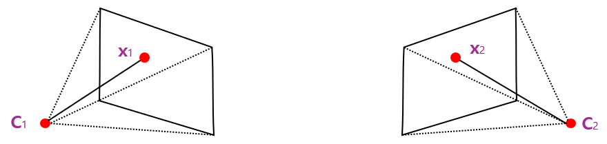
Triangulation은 2개의 카메라가 calibration 되어 있다고 가정
$P$, $P'$도 알고 $K$, $R$, $\mathbf{t}$, $K'$, $R'$, $\mathbf{t}'$을 다 알고 있음
2D corresponding point도 알고고 있다고 가정(by SIFT 알고리즘)
이렇게 대응점을 가지고 있을 때 3D point를 찾는게 Triangulation
→ 3D reconstruction
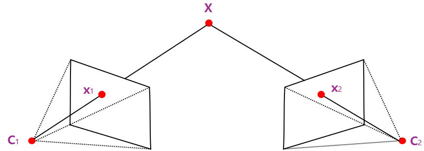
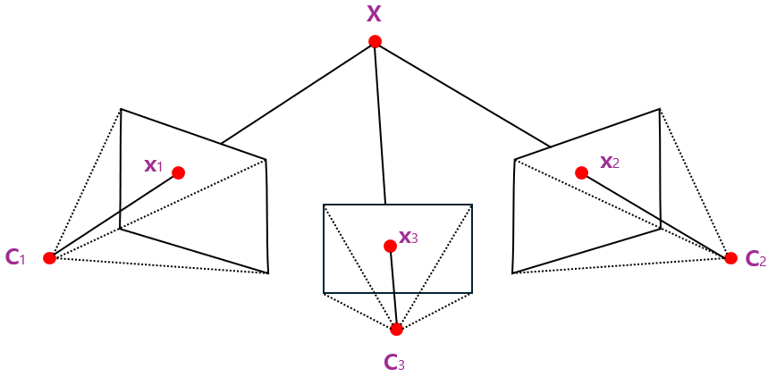
카메라가 2대 이상있어도 상관 없음
또한 여러 개의 corresponding point가 있어도 상관 없이 적용가능한 알고리즘
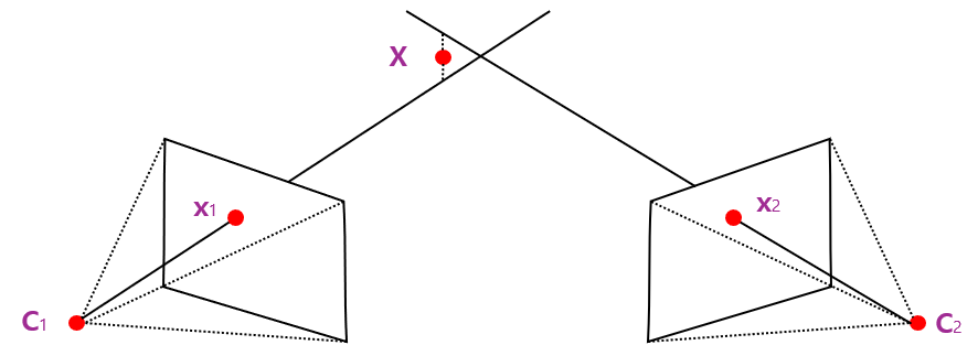
근데 대부분 3D 상에서 correspondence line들이 한 점에서 만나지 않음
→ 3D point $\mathbf{X}$를 line이 만나는 교점이라고 정의하기 어려움
→ 만나지 않는 경우가 많으니 최적의 $\mathbf{X}$를 찾아야함
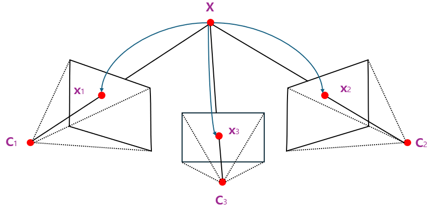
algebric하게는 $\mathbf{X}$를 찾은후 다시 projection 시켜서 모든 correspondence point $\mathbf{x}_1$, $\mathbf{x}_2$, $\cdots$가 되도록하는 최적의 값을 찾으면 됨
아마 이전부터 공부해온 내용을 떠올려보면 대충 감이 올것임 그냥 DLT를 쓰면 됨
$$\mathbf{x}_1 = P_1 \mathbf{X} = \begin{bmatrix} \mathbf{p}_1^{1T} \\ \mathbf{p}_1^{2T} \\ \mathbf{p}_1^{3T} \end{bmatrix} \mathbf{X}$$
($\mathbf{p}$: 1x4 matrix)
임의의 $\mathbf{X}$가 있다고 했을 때 위의 식을 만족
camera parameter의 행렬을 row로 분리해서 쓰면 위와 같음
$$\mathbf{x}_1 \equiv P_1 \mathbf{x}$$
그리고 up-to scale 때문에 정확한 식은 $=$ 등호가 아님
$$\lambda \mathbf{x}_1 = P_1 \mathbf{X}$$
등호로 만들어 주기 위해 up-to scale을 고려해서 $\lambda$를 사용
근데 이렇게하면 추가적인 파라미터 $\lambda$가 생기므로 파라미터를 추가하지 않기 위해
cross-product로 등호를 만들면 됨
$$\mathbf{x}_1 \times P_1 \mathbf{X} = 0$$
cross-product를 쓸 수 있는이유는 projection한 $\mathbf{x}_1$이나
ray 위를 돌아다니는 $P_1 \mathbf{X}$나 어차피 방향은 같으니 크기가 달라도 외적하면 0이 됨
$$\mathbf{x}_1 = (x_1 , y_1 , 1)^T$$
$\mathbf{x}_1$은 homogeneous coordinate
이제 외적공식에 그대로 수식 대입하면
$$x_1 (\mathbf{p}_1^{3T} \mathbf{X}) - \mathbf{p}_1^{1T} \mathbf{X} = 0$$
$$ y_1 (\mathbf{p}_1^{3T} \mathbf{X}) - \mathbf{p}_1^{2T} \mathbf{X} = 0$$
$$ x_1 (\mathbf{p}_1^{2T} \mathbf{X}) - y_1 (\mathbf{p}_1^{1T} \mathbf{X}) = 0$$
식 3개 나오는데 맨 마지막 식은 위의 2개의 식에 대해 dependent한 식이므로
결과적으로 마지막 식을 무시한채 위쪽의 2개의 식만 $\mathbf{X}$로 묶으면 다음과 같이 나옴
$$\underset{2 \times 4}{\begin{bmatrix}x_1 (\mathbf{p}_1^{3T}) - \mathbf{p}_1^{1T} \\y_1 (\mathbf{p}_1^{3T}) - \mathbf{p}_1^{2T}\end{bmatrix}} \underset{4 \times 1}{\mathbf{X}} = 0$$
이렇게 나온 식을 보면 여태까지 DLT를 썼던 $Ax=0$ 꼴이 나옴
마찬가지로 2번째 카메라 $P_2$에 대해서도 똑같이 하면 다음과 같이 나옴
$$\underset{4 \times 4}{\begin{bmatrix}x_1 (\mathbf{p}_1^{3T}) - \mathbf{p}_1^{1T} \\y_1 (\mathbf{p}_1^{3T}) - \mathbf{p}_1^{2T} \\x_2 (\mathbf{p}_2^{3T}) - \mathbf{p}_2^{1T} \\y_2 (\mathbf{p}_2^{3T}) - \mathbf{p}_2^{2T}\end{bmatrix}}\underset{4 \times 1}{\mathbf{X}} = 0$$
$$\mathbf{X}$는 4개의 변수를 가졌고 up-to scale이므로 3 DoF
만약에 카메라가 2대가 아닌 여러대가 있으면 그냥 식 더 추가해주면 됨
(카메라 $N$개가 추가 될 때마다 row가 $2N$개 씩 늘어남)
$$\underset{2N \times 4}{\begin{bmatrix}x_1 (\mathbf{p}_1^{3T}) - \mathbf{p}_1^{1T} \\y_1 (\mathbf{p}_1^{3T}) - \mathbf{p}_1^{2T} \\x_2 (\mathbf{p}_2^{3T}) - \mathbf{p}_2^{1T} \\y_2 (\mathbf{p}_2^{3T}) - \mathbf{p}_2^{2T} \\ \cdots \end{bmatrix}}\underset{4 \times 1}{\mathbf{X}} = 0$$
이제 $2N \times 4$의 왼쪽 행렬을 SVD를 한 다음에 $A=UDV^T$ 형태에서 $V^T의
마지막 column을 가져오면 그게 $\mathbf{X}$의 최적의 solution이 됨
여기 까지가 DLT로 구하는 방법이였는데 조금 문제가 있음
$$\mathbf{x}_1 \equiv P_1 \mathbf{X} \rightarrow \mathbf{x}_1 \times P_1 \mathbf{X} = 0$$
$\equiv$ 때문에 외적이란 방법을 통해 통해 0과 근사하게 해서 DLT를 풀었는데
이게 우리가 진짜 원하는 정답과 다름
무슨 말이냐면 완전히 =0이면 괜찮은데 완전히 =0이 아닐 경우가 문제인데
SVD 방법자체가 완전히 =0 이아님 근사하는 방법이고
그럼 0에 근사할 수록 실제 $\mathbf{X}$와 더 가까워지거나 들 가까워지는데
어떤게 더 좋은건지 알 수가 없음

위의 그림처럼 이상적인 $\mathbf{X}$를 projection 했더니 $\mathbf{x}_1$, $\mathbf{x}_2$하고
정확하게 만나지 않음
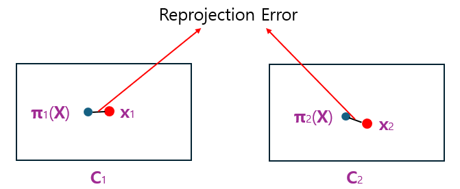
2D 상에서 보면 위와 같은 Reprojection Error가 발생하는데
우리가 원하는건 projection한 $\pi_1 (\mathbf{X})$가
우리가 input으로 넣은 $\mathbf{x}_1$, $\mathbf{x}_2$와 가까워지길 원함
식으로 표현하면 다음과 같음
$$\mathbf{X}^* = \underset{\mathbf{X}}{\text{argmin}} \, \sum_i \underset{\text{Reprojection Error}} {\| \pi_i(\mathbf{X}) - \mathbf{x}_i \|_2^2}$$
$$\text{Reprojection Error: } \left( \frac{\mathbf{P}_i^1 \mathbf{X}}{\mathbf{P}_i^3 \mathbf{X}} - x_i \right)^2 + \left( \frac{\mathbf{P}_i^2 \mathbf{X}}{\mathbf{P}_i^3 \mathbf{X}} - y_i \right)^2$$
$\pi$가 위처럼 분수형태로 나온이유는
homogeneous에서 inhomogeneous로 바꾸기 위해 마지막 요소로 나눔
어쨌든 이렇게 최소화 한 Error는 Geometric Error이고 non-linear 방법
$$\mathbf{x}_1 \equiv P_1 \mathbf{X} \rightarrow \mathbf{x}_1 \times P_1 \mathbf{X} = 0$$
맨 처음에 했던 외적 방법은 Algebraic Error를 최소화 한것이고 linear 방법
우리가 궁극적으로 원하는건 Geometric Error를 최소화 해야함
→ Geometric Error 최소화가 Reprojection Error 최소화
그래서 사용하는 방법이 initial로 맨 처음에 DLT로 구한 $\mathbf{X}$를 사용하고
이거를 가지고 Reprojection Error를 최소화하는 방향으로 gradient descent를 하면서
점점 error를 줄여나가면 됨
근데 error 줄여나갈 때 $\mathbf{X}$만 최적화 하는게 아니라 camera parameter도 최적화 함
→ SfM의 핵심기술
Triangulation은 calibration 잘 됬다고 가정하고 $\mathbf{X}$만 최적화 함
Triangulation Uncertainty
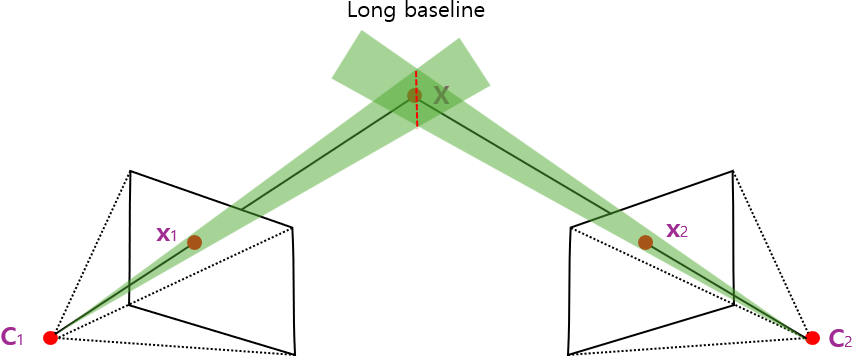
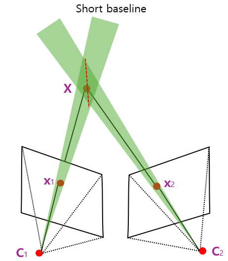
basline의 길이에 따라 Depth 오차가 달라짐
콘(Con)으로 이 오차를 확인할 수 있는데
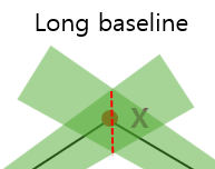
위 그림처럼 빨간색 선이 $\mathbf{X}$의 오차 범위이고 Depth uncertainty라고 부름
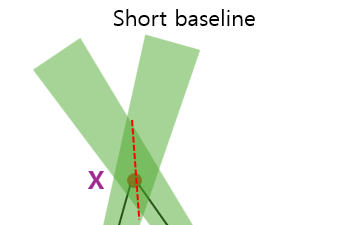
그림을 보면 알 수 있듯이 baseline이 가까울 수록 Depth uncertainty가 커짐
그러면 long baseline 선택하면 되는거 아닌가?
→ 2개의 camera view가 너무 달라 feature matching이 어려워짐
해결 책은 그냥 camera를 가운데에 하나 더 두면 됨
Correspondence
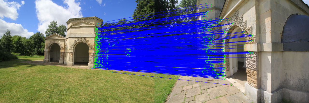
correspondence는
Homography estimation, Calibration, Fundamental/Essential matrix estimation,
3D reconstruction, ... 등에 쓰일 정도로 매우 중요한데
여태까지는 correspondence를 찾았다는 가정하에 시작했는데
사실 correspondence를 잘 찾는게 가장 중요함
찾는 방법으로는 Template matching(SSD, NCC, ...), Scale-invariant matching(SIFT, SURF, ...), Learned feature mathcing(SuperGlue, ...) 등이 있음
자세한 알고리즘 내용은 생략
Structure-from Motion(SfM)
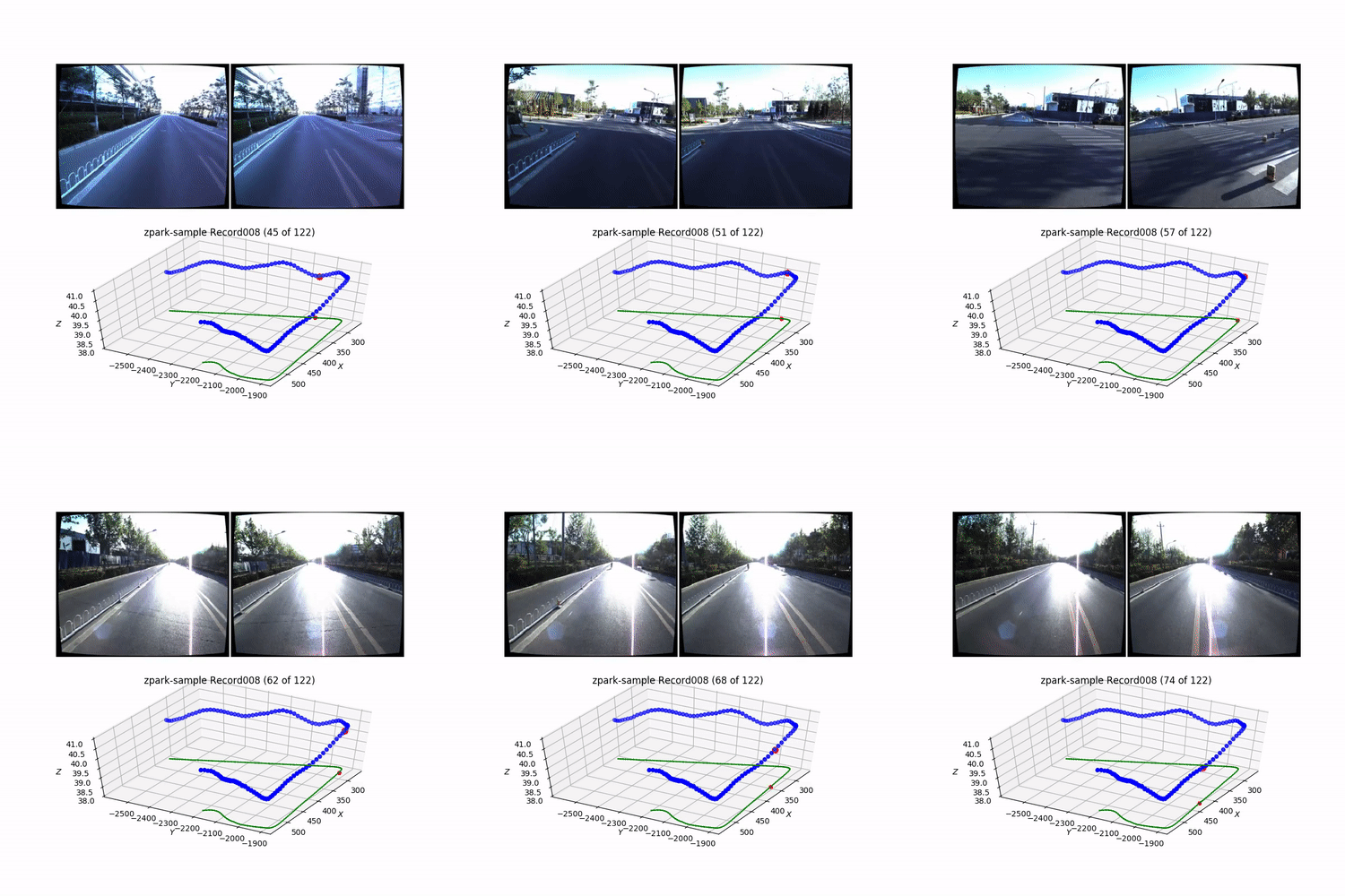
Structure-from Motion(SfM)은 Input으로 비디오나 이미지들을 막 넣으면
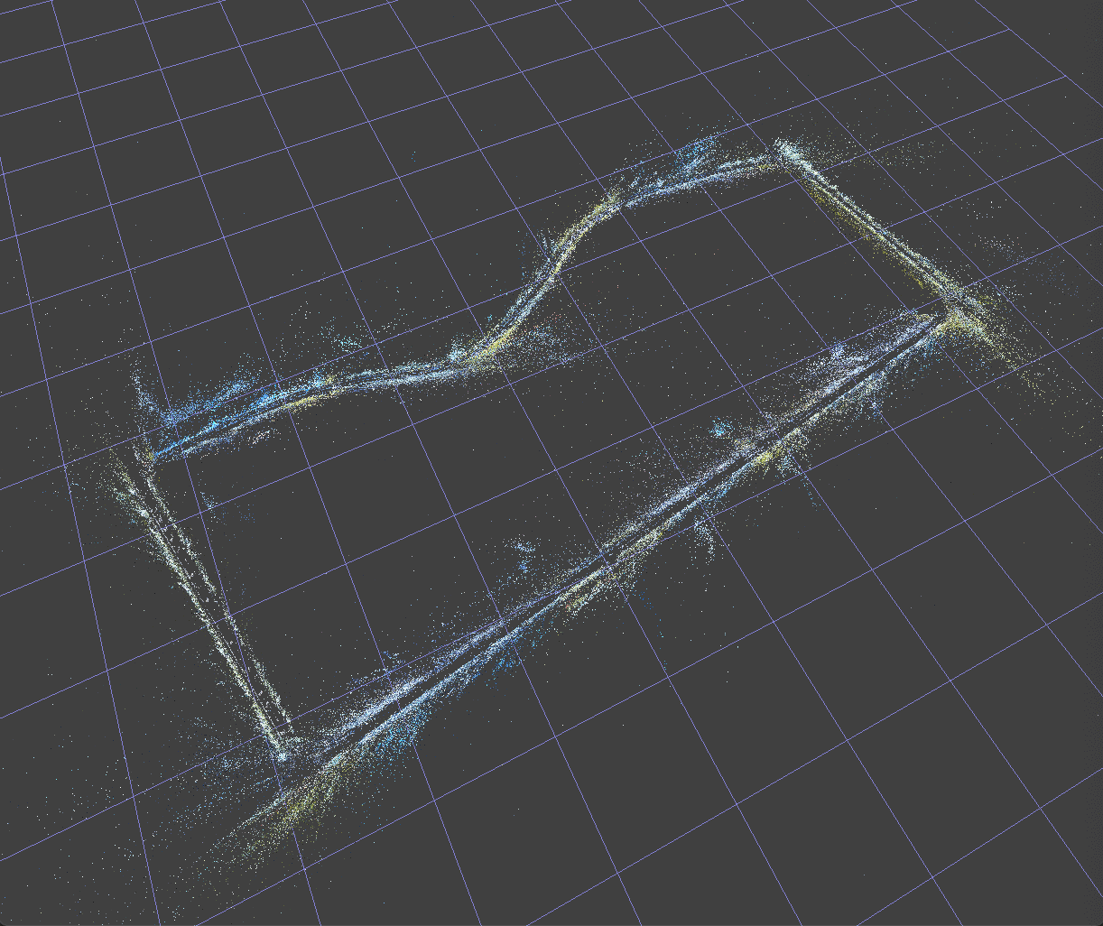
Output으로 Camera pose와 3D scene(point cloud 형태)가 나옴
다른 예시로는 인터넷상에서 어떤 건물을 수 많은 관광객들이 촬영한 이미지들을 모아서
3D scene을 재구성할수도 있음
Tomasi-Kadade Factorization(TK Factorization)
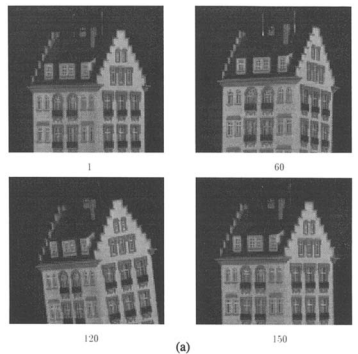
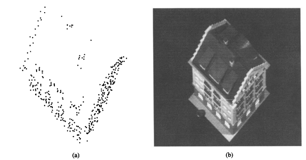
Tomasi-Kadade Factorization(TK Factorization)은 SfM의 초기 버전
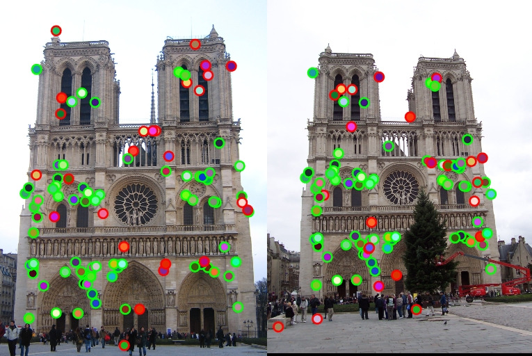
Harris corners, SIFT로 feature point를 찾고 coresspondence를 찾았다고 가정하자
먼저, SfM을 자세히 배우기전에 몇가지 Notation들을 정리해야함
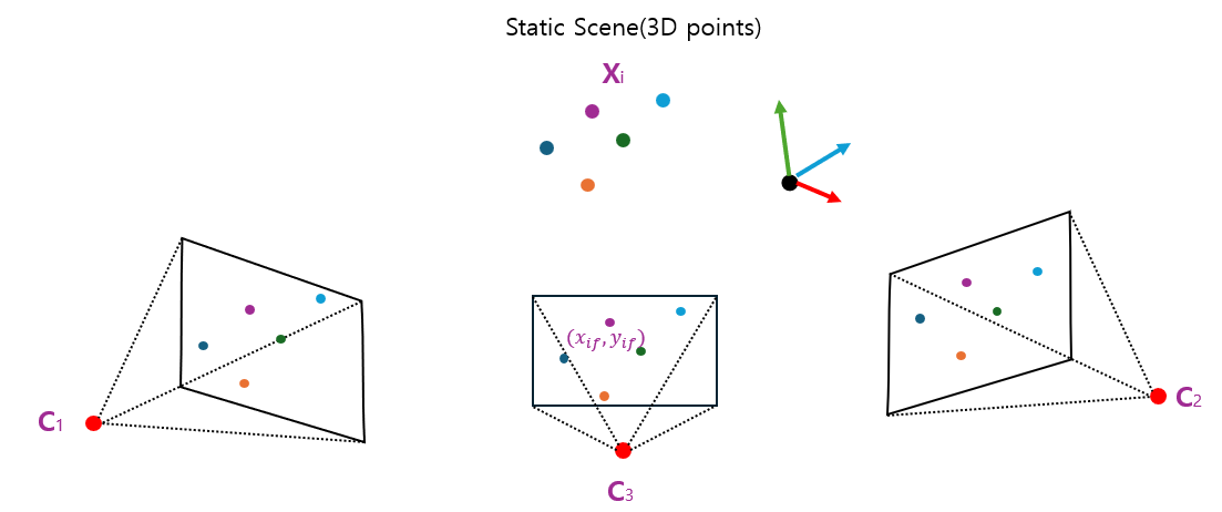
static scene에서 $i$번째 3D point를 $\mathbf{X}_i$라 하고
이에 대응되는 2D projection된 point 좌표를 $x_{if}$, $y_{if}$라 함
$i$는 point index이고 $f$는 frame index 또는 camera index
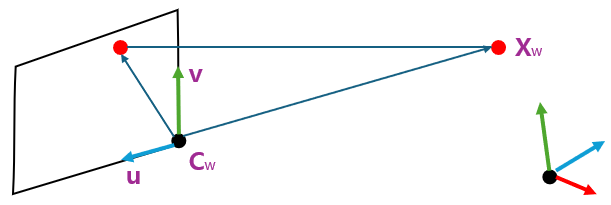
TK factorization의 가정은 다음과 같음
1) Orthographic Projection
$K$가 없음 그냥 $z$ 없애서 수직으로 projection
camera orientation을 $\mathbf{u}$, $\mathbf{v}$로 표현함
→ camera parameter의 $R$과 같음
camera center world coordinate가 $\mathbf{C}^w$
따라서, projection된 $x$, $y$를 구하려면 그냥 $\mathbf{u}$, $\mathbf{v}$와 내적하면 됨
$$x = \mathbf{u}^T \mathbf{X}^c = \mathbf{u}^T (\mathbf{X}^w - \mathbf{C}^w )$$
$$y = \mathbf{v}^T \mathbf{X}^c = \mathbf{v}^T (\mathbf{X}^w - \mathbf{C}^w )$$
2) Camera center world coordinate를 3D points들의 중심으로 설정
$$\frac{1}{N} \sum_{i=1}^N \mathbf{X}_i = 0$$
camera center를 중심으로 모든 3D points $\mathbf{X}$들을 더하면 위의 식을 만족함
$$x_{if} = \mathbf{u}^T (\mathbf{X}_i - \mathbf{C}_f)$$
$$y_{if} = \mathbf{v}^T (\mathbf{X}_i - \mathbf{C}_f)$$
2D correspondence $(x_{if} , y_{if})$는 주어졌다고 가정했고
3D points $\mathbf{X}_i$를 찾아야함
그런데 camera pose(position) $\mathbf{C}_f$를 모르고,
camera orientation $\mathbf{u}$, $\mathbf{v}$도 모름
(카메라의 방향은 $\mathbf{u}$, $\mathbf{v}$를 외적하면 구할 수 있음)
$\mathbf{C}_f$에는 $R$, $\mathbf{t}$ 성분이 있고, $\mathbf{u}$, $\mathbf{v}$에도 $R$ 성분이 있음
사실 $\mathbf{C}_f$는 Orthographic Projection 때문에 depth가 의미가 없어서 필요가 없음
그래서 위의 식에서 $\mathbf{C}_f$를 식에서 없애는게 첫번째 해야할 고민임
이를 위해 몇가지 트릭을 사용함
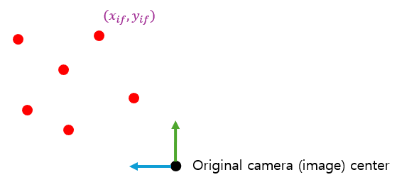
$$\hat{x}_{if} = x_{if} - \frac{1}{N} \sum_{j=1}^N x_{jf} = x_{if} - \bar{x}_f$$
$$\hat{y}_{if} = y_{if} - \frac{1}{N} \sum_{j=1}^N y_{jf} = y_{if} - \bar{y}_f$$
각 $f$번째 frame마다 2D points들의 center $\bar{x}_f$, $\bar{y}_f$를 구함
그런다음 이렇게 구한 center를 기준으로 나머지 모든 2D points들의 좌표를 새로 구성
→ 그렇게 만든게 $\hat{x}_{if}$, $\hat{y}_{if}$
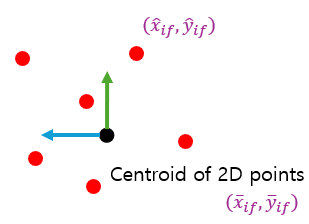
$x_{if}$, $y_{if}$는 이미 알고 있으니 나머지 center 좌표나 새로운 좌표도 다 구할 수 있음
이제 수식을 전개해보면
$$\begin{align*}\hat{x}_{if} &= x_{if} - \frac{1}{N} \sum_{j=1}^{N} x_{jf} \\&= \mathbf{u}^T_f \left( \mathbf{X}_i - \mathbf{C}_f \right) - \frac{1}{N} \sum_{j=1}^{N} x_{jf} \\&= \mathbf{u}^T_f \left( \mathbf{X}_i -\mathbf{C}_f \right) - \frac{1}{N} \sum_{j=1}^{N} \mathbf{u}^T_f \left( \mathbf{X}_j - \mathbf{C}_f \right) \\&= \mathbf{u}^T_f \left( \mathbf{X}_i - \mathbf{C}_f \right) - \mathbf{u}^T_f \underbrace{\frac{1}{N} \sum_{j=1}^{N} \mathbf{X}_j}_{=0} +\mathbf{u}^T_f \mathbf{C}_f \\&= \mathbf{u}^T_f \mathbf{X}_i\end{align*}$$
수식 전개과정에서 3번째줄
$ - \frac{1}{N} \sum_{j=1}^{N} \mathbf{u}^T_f \left( \mathbf{X}_j - \mathbf{C}_f \right)$은
$j$랑 관련없는 $\mathbf{u}^T_f$와 $\mathbf{C}_f$는 상수취급 후 전개
4번째줄에서 마지막항은 $N \times \frac{1}{N}$으로 1이되서 $\mathbf{u}^T_f \mathbf{C}_f$만 남고
$\frac{1}{N} \sum_{j=1}^{N} \mathbf{X}_j$은 처음에 가정2에서 3D points들의 중심을 origin으로 가정했기 때문에 0이됨
결국 전개해서 나온 결과를 보면 $\mathbf{C}_f$가 없는 $\mathbf{u}^T_f \mathbf{X}_i$가 됨
마찬가지로 $y$도 똑같이하면 다음과 같은 결과가 나옴
$$\hat{x}_{if} = \mathbf{u}^T_f \mathbf{X}_i$$
$$\hat{y}_{if} = \mathbf{v}^T_f \mathbf{X}_i$$
$$\begin{bmatrix} \hat{x}_{if} \\ \hat{y}_{if} \end{bmatrix} = \begin{bmatrix} \mathbf{u}^T_f \\ \mathbf{v}^T_f \end{bmatrix} \mathbf{X}_i$$
3)
마지막 3번째 가정인데 TK에서는 모든 3D points가 모든 이미지에서 projection된걸 볼 수 있다고 가정
이제 이 수식과 가정3을 통해 모든 points에 대해서 행렬식을 만들 수 있음
$$\underset{\mathbf{W}_{2F \times N}}{\begin{bmatrix}\hat{x}_{11} & \hat{x}_{21} & \cdots & \hat{x}_{N1} \\\hat{x}_{12} & \hat{x}_{22} & \cdots & \hat{x}_{N2} \\\vdots & \vdots & \ddots & \vdots \\\hat{x}_{1F} & \hat{x}_{2F} & \cdots & \hat{x}_{NF} \\\hdashline \hat{y}_{11} & \hat{y}_{21} & \cdots & \hat{y}_{N1} \\\hat{y}_{12} & \hat{y}_{22} & \cdots & \hat{y}_{N2} \\\vdots & \vdots & \ddots & \vdots \\
\hat{y}_{1F} & \hat{y}_{2F} & \cdots & \hat{y}_{NF}\end{bmatrix}} = \underset{\mathbf{M}_{2F \times 3}}{\begin{bmatrix} \mathbf{u}^T_1 \\ \mathbf{u}^T_2 \\ \vdots \\ \mathbf{u}^T_F \\ \mathbf{v}^T_1 \\ \mathbf{v}^T_2 \\ \vdots \\ \mathbf{v}^T_F \end{bmatrix}} \underset{\mathbf{S}_{3 \times N}}{\begin{bmatrix} \mathbf{X}_1 & \mathbf{X}_2 & \cdots & \mathbf{X}_N \end{bmatrix}}$$
$\mathbf{W}_{2F \times N}$ 행렬을 보면
row는 위에서부터 Frame1 ~ Frame F 이후 다시 Frame 1 ~ Frame F이고
column은 Point 1 ~ Point N임
재밌는건 Centroid-subtracted 2D points matrix($\mathbf{W}_{2F \times N}$)의 모든 좌표 값을
알고 있기 때문에 이 행렬을 구한 후 분해하면 Camera motion matrix($\mathbf{M}_{2F \times 3}$)나 3D points matrix($\mathbf{S}_{3 \times N}$)를 알 수 있음 그래서 TK factorization이라 부름
그리고 Camera motion matrix는 $2F \times 3$, 3D points matrix $3 \times N$인데
3이라는 숫자가 고정되어 있음
이 말은 두 행렬 모두 Rank가 3이 최대이고 matrix 2개의 곱도 Rank 3이 최대
$$\text{Rank}(\mathbf{W}) \le \text{min}(\text{Rank}(\mathbf{M}) ,\ \text{Rank}(\mathbf{S})) = 3$$
point에 noise가 있으면 $\mathbf{W}$가 Full-Rank 일 수도 있음
일단은 Rank=3이 되도록 $\mathbf{W}$를 SVD를 통해 decompose를 하면 됨

가운데 $D$행렬에서 파란색 부분이 전부 0이여야 함
만약 $\mathbf{W}$가 노이즈가 껴서 0이 아니면 강제로 0으로 만든 다음 다시 $UDV^T$를 곱해서
$\tilde{\mathbf{W}}$를 만들어줌
그런다음 다시 SVD로 분해한 후 행렬에서 0인 부분을 전부 없애버리면 아래처럼 간략화가 가능함
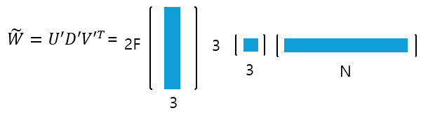
그런다음 이제 $D$의 대각성분에 root를 사용해 행렬을 2개로 나눠줌
$$\tilde{\mathbf{W}} = \underset{2F \times 3}{U'} \underset{3 \times 3}{D^{' \frac{1}{2}}} \underset{3 \times 3}{D^{' \frac{1}{2}}} \underset{3 \times N}{V^{'T}}$$
여기까지하면 $U'D^{' \frac{1}{2}}$은 $\mathbf{M}_{2F \times 3}$이고 $D^{' \frac{1}{2}} V^{'T}$은 $\mathbf{S}_{3 \times N}$일 수도 있지만 이것이 유일한 solution도 아니고 정확한 답이 아닐 수도 있음
따라서, 가운데에 임의의 $Q$ 행렬을 곱해주는데
$$\tilde{\mathbf{W}} = \underset{2F \times 3}{U'} \underset{3 \times 3}{D^{' \frac{1}{2}}} \underset{3 \times 3}{Q} \underset{3 \times 3}{Q^{-1}} \underset{3 \times 3}{D^{' \frac{1}{2}}} \underset{3 \times N}{V^{'T}}$$
이제 적절한 $Q$를 찾으면 됨
여기까지 계산하면서 유일하게 안 쓴 조건이 하나 있는데
$$\mathbf{W}_{2F \times N} = \underset{\mathbf{M}_{2F \times 3}}{\begin{bmatrix} \mathbf{u}^T_1 \\ \mathbf{u}^T_2 \\ \vdots \\ \mathbf{u}^T_F \\ \mathbf{v}^T_1 \\ \mathbf{v}^T_2 \\ \vdots \\ \mathbf{v}^T_F \end{bmatrix}} \underset{\mathbf{S}_{3 \times N}}{\begin{bmatrix} \mathbf{X}_1 & \mathbf{X}_2 & \cdots & \mathbf{X}_N \end{bmatrix}}$$
$\mathbf{M}_{2F \times3}$에서 $\mathbf{u}$랑 $\mathbf{v}$가 서로 orthogonal 해야 함
$$U'D^{' \frac{1}{2}} Q = \begin{bmatrix}\tilde{\mathbf{u}}_1^T \\\tilde{\mathbf{u}}_2^T \\\vdots \\\tilde{\mathbf{u}}_F^T \\\hdashline\tilde{\mathbf{v}}_1^T \\\tilde{\mathbf{v}}_2^T \\\vdots \\\tilde{\mathbf{v}}_F^T\end{bmatrix} Q$$
여기서 $U'D'^{\frac{1}{2}}$를 곱해서 matrix를 만든 후 그걸 $Q$랑 곱했을 때 아래조건 만족해야함
$$\mathbf{u}^T_f \mathbf{u}_f = 1$$
$$\mathbf{v}^T_f \mathbf{v}_f = 1$$
$$\mathbf{u}^T_f \mathbf{v}_f = 0$$
따라서, $\mathbf{u}^T_f = \tilde{\mathbf{u}}_f^T Q$이고 $\mathbf{u}_f = Q^T \tilde{\mathbf{u}}_f$이므로
이거를 위에 대입해주면 아래처럼 됨
$$\begin{aligned}\tilde{\mathbf{u}}_f^T Q Q^T \tilde{\mathbf{u}}_f &= 1 \\\tilde{\mathbf{v}}_f^T Q Q^T \tilde{\mathbf{v}}_f &= 1 \\\tilde{\mathbf{u}}_f^T Q Q^T \tilde{\mathbf{v}}_f &= 0\end{aligned}$$
마찬가지로 방정식이 나왔으니 DLT로 풀어서 조건을 만족하는 $Q$를 찾으면 됨
TK Factorization은 아주 좋은 알고리즘이지만
가정이 여러개 있다는 점에서 Computer vision에서 지금은 안 쓰임
'3D Computer Vison' 카테고리의 다른 글
| [3D CV] SfM & Bundle Adjustment (0) | 2025.01.20 |
|---|---|
| [3D CV] Two View Geometry (2) (2) | 2025.01.17 |
| [3D CV] Two View Geometry (1) (0) | 2025.01.16 |
| [3D CV] PnP (0) | 2025.01.16 |
| [3D CV] More single view (1) | 2025.01.15 |


